We have moved to a new website. You are being redirected!

This week’s write up is a little more personal than our usual topics. I thought it would be interesting to measure my work-life balance over time by plotting my billable hours since I started working. I work for a boutique financial advisory firm that specializes in infrastructure and energy finance. We mainly advise governments so our hours can be a little lighter than other finance professionals, but I remember my hours being pretty brutal when I first started. The last few years have been more reasonable. Let's see if my time sheets tell the same story.

Tracking billable hours is one of the most tedious aspects of client-based work, as anyone who has had to fill out time sheets can attest. As it happens, I have saved (almost) all of my time sheets since I started working my current job back in April 2009 in Word Document tables. That’s about 79 time sheets.

The source code for the data analysis can be found here.

We can start by plotting weekly billable hours since April 2010, when I started working as a permanent, full-time employee. As shown in Figure 1 below, there is significant variability in my hours from week to week, but the trend appears to suggest a gradual decrease in hours over time. Let’s smooth out the week to week variability by calculating rolling averages.

Figure 1. Weekly Billable Hours

Figure 2 below shows weekly billable hours on a four and sixteen week moving average basis. The pattern is clearer when we smooth out the week to week variability. I've been billing fewer and fewer hours since I started working, although the decrease is more muted if you exclude 2011, which was an unusually busy year. If my bosses read this, I would just remind them that billing and productivity are not necessarily the same thing.

Figure 2. Weekly Billable Hours (Moving Average)

Figure 3 shows a frequency distribution of weekly billable hours along with summary statistics. I bill 43.8 hours per week on average with a standard deviation of 11.8 hours. A quarter of the time, I bill 51 or more hours per week. The busiest week was 79 hours.

Figure 3. Distribution of Weekly Billable Hours

I was also curious to know if the week to week variability in my hours has changed over time. To measure this variability, I calculated the standard deviation of billable hours over rolling four week periods. I then smoothed out the figures by calculated a sixteen week moving average of the four week standard deviations. The result is shown in Figure 4. While it appears as though the variability has decreased over time, the results are distorted by a spike in 2011. Excluding the spike in 2011, the variability is unchanged. My schedule is still generally unpredictable. In fact, the standard deviation over the last four weeks was in the top 15th percentile historically (including the spike in 2011).

Figure 4. Standard Deviation of Billable Hours (Moving Average)

(including spike in 2011)

(excluding spike in 2011)

We have moved to a new website. You are being redirected!

A couple of weeks ago, Stromae performed at a sold out show in Washington, DC. Several friends were scouring StubHub and Craigslist for tickets, but ticket prices seemed to be all over the place. That got us wondering whether the market price for concert tickets exhibits any patterns that can be used to improve your chances of getting the best price (highest, if you’re the seller; lowest, if you’re the buyer).

First, we needed a dataset of market transactions for concert tickets. As it turns out, StubHub provides this data to help sellers determine a listing price. Unfortunately, StubHub would not provide us with a dataset of sold ticket prices so we had to manually scrape their website over the course of a couple of weeks. Our dataset includes 16,562 ticket sales from 32 concerts in 17 cities and from 20 different artists. We started out with more than 20,000 ticket sales but remove transactions that occurred earlier than 90 days before the show, as well as the top and bottom 5th percentiles to remove outliers in the data.

The source code for the analysis can be found here. We usually provide the dataset but, in this case, we’ll need StubHub's approval to share the data that we scraped from their website.

Grouping and Standardizing Ticket Prices

Since ticket prices vary by city, show, seating section, date, etc., the first challenge was to group the raw data into categories in order to compare the 16,562 data points that we have in a meaningful way. We’re interested in the change in ticket prices for each seating section as the date of the show approaches, so we grouped the data by section (e.g., ‘Ed Sheeran / New York / Orchestra 201’ would be one section) with the timeline being the number of days before the show.

A second challenge was to scale or standardize ticket prices whose absolute dollar value varies significantly from section to section. After all, we are interested in the movement of prices over time and not their absolute dollar value. To standardize the prices, we used z-score scaling, which transforms each ticket price into a value that represents its position (percentile rank) within its section assuming a normal distribution of prices. In other words, the average/mean ticket price in each section will have a value of zero and the standard deviation of prices in each section will be one (meaning that 95% of ticket prices in each section will have a z-score between -1.96 and 1.96). This makes it easier to compare the relative movement of ticket prices across sections because now prices in each section have the same scale (roughly -2.0 to 2.0, with an average of zero), instead of an absolute dollar value (which, in our case, ranges from a few dollars to more than $500, with different averages for each section).

Figure 1 shows the impact of z-score scaling on the distribution of the ticket prices in our dataset. As you can see, z-score scaling standardizes the ticket prices by converting them into a normal distribution with mean zero and standard deviation of one. This allows us to compare ticket prices across sections as the average ticket price in each section will be zero and the distribution of ticket prices will be the same.

Figure 1. Ticket Price Frequency Distribution

Ticket Price Pattern

Now that we’ve grouped and standardized the ticket price data, we can start observing patterns. Figure 2 shows the average ticket price z-score during the 90 days before a show, converted into the relevant percentile rank. The blue shaded area shows the 95% confidence interval. One way to interpret the chart below is: 55 days before a show (x-axis), the average ticket price (across sections) is in the 50th percentile (y-axis) of prices for tickets sold in that section during the entire 90 day period. The red dotted line is a best fit curve.

Figure 2. Ticket Price Pattern

From the period between 90 and 30-35 days before a show, ticket prices tend to gradually increase, peaking about 30-35 days before a show. After that, prices start to fall until the day of the show. We suspect that this pattern is the result of people’s scheduling habits. Between 90 and 30 days before a show, demand grows as people start planning to attend a show and go purchase tickets from the market. Supply, on the other hand, is limited, as most ticketholders also plan to attend the show. In the last 30 days, the price is driven down by an increase in the supply of tickets as unexpected schedule conflicts force people who had previously planned to attend a show to sell their tickets.

Based on the pattern above, the best time to buy a concert ticket is about 55 days before a show (the earlier the better). If that time has passed, then you’re better off waiting until the day of the show to buy your ticket as prices are likely to gradually fall over the last 30-35 days. On the day of the show, ticket prices are on average as low as they were about 55 days before the show.

If you’re a seller, you’re most likely to get the highest price for your ticket 30-35 days before the show. If you’re looking to sell in the last 30 days (because of an unexpected schedule conflict?), you should do so right away. The price is likely to continue falling until show time.

We have moved to a new website. You are being redirected!

Earlier this week, we examined the surge in D.C.’s crime rate in 2015. We discovered that, as of August 2015, D.C.’s monthly homicide rate had more than doubled from the 2011 to 2014 average. Since 2011, there had been only one month when D.C.'s murder rate reached as high as 16 victims. There have been 16 or more murders in every month since May of this year (including 14 so far in August).

In this write-up, we’ll examine the violent crime rate within Wards and neighborhood clusters, and rank the most improved and most regressed neighborhoods. The data shows that just three neighborhoods account for nearly 80 percent of the increase in the murder rate so far this year.

D.C.’s crime incidents data can be found here. The source code for the data analysis can be found here. The murder of 23-year old Matthew Castrol Shlonsky on August 16, 2015 in the Shaw neighborhood of Northwest D.C. did not appear to be reported in the crime incidents data. We have manually added it.

Homicides by Ward

Let’s take a look at the annual homicide rate by Ward (Figure 1). For those of you less familiar with D.C.'s geography, here's a boundary map of each Ward. Since we’re only halfway through 2015, the charts below only consider crimes reported between January and August 19 of each calendar year (rather than the entire calendar year). We’ve excluded Ward 3 because there are not enough data points in that area to create a meaningful chart (although the murder rate there has increased between 2014 and 2015). 

Murders are up in every Ward, except 1 and 7, with Ward 8 registering the largest increase. While D.C.'s homicide rate has clearly increased between 2014 and 2015, the rate appears to have begun its increase in 2013 and not 2014. Only Ward 7 experienced a significant decrease in homicides between 2014 and 2015.

Figure 1. Homicides by Ward

The increase in the homicide rate in Ward 8 is equal to just under half of the net increase in the number of murders between 2014 and 2015. The increases in Wards 3 and 5 each make up about 18 percent. Within each Ward, specific neighborhoods have been affected more than others.

Using D.C.'s neighborhood cluster classification, we can calculate the change in the murder rate on a neighborhood by neighborhood basis. The largest increase in murders between 2014 and 2015 occurred in Woodland/Fort Stanton, Garfield Heights, Knox Hill (Ward 8, +8 murders), Douglass, Shipley Terrace (Ward 8, +8 murders), and Shaw, Logan Circle (Ward 2, +5 murders). These three neighborhoods account for 80 percent of the increase in the murder rate so far this year.

The most improved neighborhoods are Sheridan, Barry Farm, Buena Vista (Ward 8, -6 murders) and Deanwood, Burrville, Grant Park, Lincoln Heights, Fairmont Heights (Ward 7, -4 murders).

Non-Homicide Violent Crimes by Ward

Has the increase in murders been accompanied by an increase in other violent crimes? Figure 2 below shows the annual violent crime rate by Ward for the January to August 19 period for each calendar year. It is interesting to note that while Ward 8 appears to have registered the largest increase in homicides from 2014 to 2015, violent crime excluding murders is actually down. A similar observation can be made of Ward 1, 2 , and 3. Ward 7 is the only one to experience a drop in both homicides and other violent crimes.

Figure 2. Other Violent Crimes by Ward

Relationship between Homicide and Other Violent Crimes

Figure 3 attempts to measure the relationship between the change in homicides and the change in other violent crimes on a neighborhood by neighborhood basis between 2014 and 2015. Counterintuitively, the correlation is nearly zero. There appears to be no relationship between the change in homicides and the change in other violent crimes. In fact, nearly 40 percent of neighborhoods experienced an improvement in one rate and a regression in the other. The correlation was stronger in 2011-2013, but began breaking down in 2013, indicating that there may have been a structural change in the drivers of D.C.'s homicide rate after 2013. It is difficult to draw any conclusions with only five years of data but it is an area worth additional examination.

Figure 3. Relationship Between Change in Homicides and Other Violent Crimes

Most Improved and Most Regressed Neighborhoods

As we noted above, Ward 7 has seen the most improvement among all of the wards, registering significant drops in both homicides and other violent crimes between 2014 and 2015. Chart-it has also ranked D.C. neighborhoods by the largest increase and decrease in violent crimes between 2014 and 2015. We excluded the bottom 20th percentile to prevent neighborhoods with a very low crime rate from distorting the ranking.

Figures 4 shows the top ten most regressed neighborhoods. The top ranked neighborhood is in Ward 4. The next two are in Wards 1 and 5, respectively.

Figure 4. Top 10 Most Regressed Neighborhoods between 2014 and 2015

Rank	Neighborhood	Increase (pct)	Increase (Incidents)	Avg Annual Violent Crime Incidents *
1	Lamond Riggs, Queens Chapel, Fort Totten, Pleasant Hill	49	24	56
2	Kalorama Heights, Adams Morgan, Lanier Heights	49	23	84
3	Brookland, Brentwood, Langdon	38	35	119
4	Takoma, Brightwood, Manor Park	33	28	103
5	NoMa, Union Station, Stanton Park, Kingman Park	33	53	187
6	Ivy City, Arboretum Trinidad, Carver Langston	23	46	205
7	Capitol Hill, Lincoln Park	20	22	117
8	Edgewood, Bloomingdale, Truxton Circle, Eckington	19	27	157
9	Twining, Fairlawn, Randle Highlands, Penn Branch, Fort Davis Park, Dupont Park	18	21	134
10	Dupont Circle, Connecticut Avenue/K Street	15	11	111

* Average Annual Violent Crime incident only includes period from January to August 19 of the period 2011 to 2015.

Figure 5 shows the top ten most improved neighborhoods. Not surprisingly, the top three are in Ward 7. Congratulations to Ward 7 for bucking the trend and becoming an overall safer place. 

Figure 5. Top 10 Most Improved Neighborhoods between 2014 and 2015

Rank	Neighborhood	Decrease (pct)	Decrease (Incidents)	Avg Annual Violent Crime Incidents *
1	Eastland Gardens, Kenilworth	-68	-28	22
2	Fairfax Village, Naylor Gardens, Hillcrest, Summit Park	-41	-16	36
3	River Terrace, Benning, Greenway, Fort Dupont	-24	-45	160
4	Sheridan, Barry Farm, Buena Vista	-21	-22	115
5	Howard University, Le Droit Park, Cardozo/Shaw	-18	-20	139
6	Southwest Employment Area, Southwest/Waterfront, Fort McNair, Buzzard Point	-17	-9	60
7	Georgetown, Burleith/Hillandale	-12	-4	31
8	West End, Foggy Bottom, GWU	-12	-3	24
9	Mayfair, Hillbrook, Mahaning Heights	-11	-13	91
10	Capitol View, Marshall Heights, Benning Heights	-8	-24	186

* Average Annual Violent Crime incident only includes period from January to August 19 of the period 2011 to 2015.

We have moved to a new website. You are being redirected!

What is happening in DC this summer? The City appears to be in the midst of a crime surge with a new high-profile shooting, stabbing, or violent assault every week. Does the crime data support this observation? This post will examine the DC crime rate so far this year compared to the rate during the last five years.

DC’s crime incidents data can be found here. The source code for the data analysis can be found here.

DC Violent Crime Rate

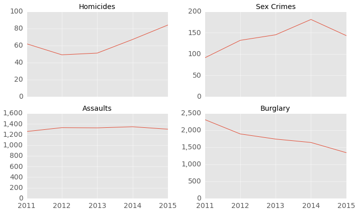
Let’s take a look at the annual crime rate of four key types of violent crime reported by Metro PD: homicides, sex crimes, assaults with a deadly weapon and burglaries. Since we’re only halfway through 2015, the charts below only consider crimes reported between January and July of each calendar year (rather than the entire calendar year). The number of homicides is up since hitting a recent annual low in 2012. Other violent crimes, however, are down so far in 2015. Let’s take a closer look at the homicide rate.

Figure 1. DC Violent Crime Incidents by Year (January to July of Every Year)

DC Homicide Rate

Figure 2 below shows the monthly homicide rate from January 2011 to July 2015 (the last month in 2015 for which a full month of data is available).  The number of homicides seems to have increased in 2015. However, it's difficult to get a sense for the overall trend given the volatility in the number of homicides in any given month (not surprising given the low number of data points).

Figure 2. Monthly Homicide Rate (January 2011 to July 2015)

We can smooth out the month-to-month variability by calculating the monthly rate on a 3-month rolling average basis (Figure 3 below). It is clear that DC's homicide rate has surged in 2015 compared to the period from 2011 to 2014, and the increase hasn’t been a one-off monthly increase but a sustained multi-month jump that shows no sign of letting up. The monthly homicide rate has jumped from about eight per month on average from 2011-2014 to about 12 per month on average so far in 2015 (from January to August), and to 17 per month as of today (August 2015).

Figure 3. Monthly Homicide Rate (Rolling 3-Month Average)

As of August 2015, DC’s average monthly homicide rate is more than twice as high as the average rate during the period from 2011 to 2014.  At this pace, DC is set to exceed 180 murders in 2015, compared to 92 reported in 2013 (excluding the 12 killed during the Navy Yard shooting).  The last time DC's homicide rate exceeded 180 was in 2008, before the City succeeded in cutting the murder rate in half between 2008 and 2013 to a multi-decade low. Could the homicide rate just be reverting to the mean?

We have moved to a new website. You are being redirected!

The 2015 NBA finals between the Cleveland Cavaliers and the Golden State Warriors has been one of the most exciting series in recent years.  The underdog Cleveland Cavaliers are up 2-1 and game four is scheduled for tonight.  In this write-up, chart-it looks at each player's share of their team's total points scored and total salary.  You can find the data used in this write-up here and here.  The source code for the data analysis can be found here.

LeBron’s importance to the Cavs has been widely discussed, particularly in light of injuries that will force three of the Cavs starters to miss the finals.  The 2015 NBA finals are essentially LeBron James versus the Warriors. But just how important is he?  Let’s look at points scored by each player in Figure 1 below. LeBron has scored more than 42 percent of the team’s points during the first three games of the series. The next highest is Timofey Mozgov, who’s scored just over 13 percent of the team’s points.  Mathew Dellavedova, a key player for the Cavs during the series, has scored 10 percent of the team’s total points.

The Warriors points are more evenly distributed with both Steph Curry and Klay Thompson each scoring about a quarter of the team’s points.  Andre Iguodala is in third place with 12.7 percent.

Figure 1.   Points Scored

Points scored understates LeBron’s contribution to team scoring as he’s also leading the Cavs in assists, averaging more than eight per game during the finals.  Looking at points scored directly by LeBron and points scored because of LeBron’s assists, he’s been involved in close to 60 percent of the team’s total points.  Curry is responsible for close to 38 percent of the Warrior's points.  Klay Thompson, with just four assists all series, has not contributed much by way of assist points.  In general, the Warriors have lagged the Cavs in assists, with the entire team logging about 48 assists compared to the Cavs' 61.

Figure 2.   Points Scored and Assist Points

For fun, we also looked at each player’s share of their respective team’s total salary.  The Cavs are currently fielding players who make up just 62.5 percent of their team’s total salary, which helps put into perspective the magnitude of the team’s injuries.  In fact, the 62.5 percent includes Kyrie Irving, who was injured in Game 1 of the finals.  Without Kyrie, the Cavs players make up about 54 percent of the team’s total salary.  By comparison, the Warriors players comprise 94.4 percent of the team’s salary.

Also interesting is that David Lee (who sat on the bench for most of the season and playoffs) is currently the highest paid player on the Warriors roster, earning 50 percent more than Steph Curry, the league MVP.  In fact, Curry isn’t even the second (Andrew Bogut) or third (Andre Iguodala) highest earner on the team. Curry’s $10.6 million salary, about half of what LeBron earns, ranks him fourth among his teammates.  Curry is clearly underpaid.  But Klay Thompson, who's scored as many points as Curry during the finals, may be even more underpaid.  His $3.1 million salary puts him near the bottom of the team’s salary ranking.  Don't feel bad for Klay though.  Under his new contract, he'll be making upwards of $15 million a year starting next year, making him the team's highest paid player, at least until 2017, when Curry's contract expires.  The Warriors salary distribution is relatively even, with four players each accounting for 14-20 percent of the team’s total salary. 

The Cavs have a more lopsided salary distribution with LeBron earning 40 percent of the total salary among players fielded by the Cavs in the finals (46 percent excluding Kyrie and 25 percent of the total Cavs salary).  Dellavedova’s salary is just under a million dollars, the lowest salary among all of the players who have played this series.

Figure 3.   Player Salaries **

**  The left column under "% Total" is the player's share of the total salary of the selected players (i.e., players who have been active during the finals). The right column is the player's share of the team's total salary.